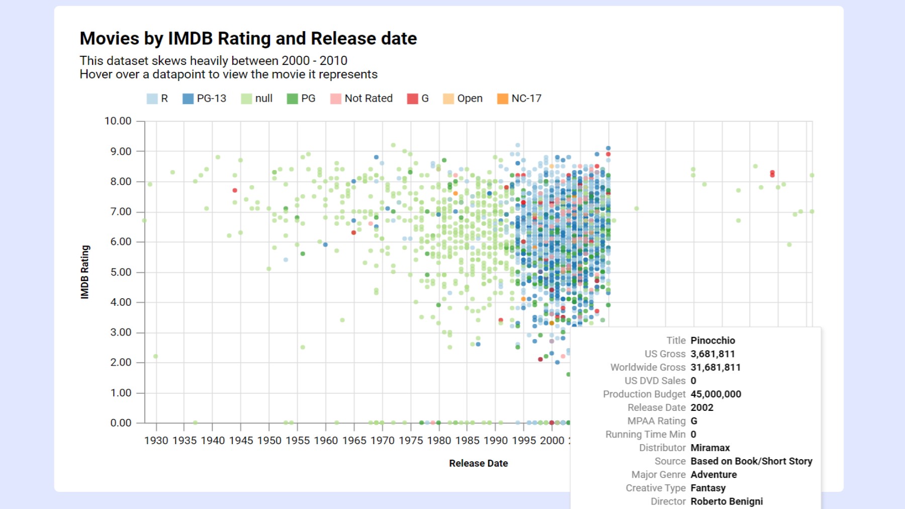
How to create a chart from an excel file
Upload an Excel workbook to InstaCharts to instantly generate a chart from your data


Create charts from excel files
InstaCharts lets you create a chart from an Excel file, change the chart’s axis or type without manually reselecting data in your spreadsheet, and share the result with a coworker.
TLDR: Try the demo or sign up for a free account!
1. Load your Excel file
 View your excel spreadsheet data on the Data Tab
From your workspace, click New, then New Sheet, and choose Upload a file, or drag and drop the file onto the workspace. InstaCharts opens Excel files in the .xlsx, .xls, .xlsm and .xlsb formats. An import preview shows the first 100 rows, with each column header color coded by the type InstaCharts detected: green for dates, blue for numbers, and pink for text. InstaCharts will auto detect the column type for each column in the spreadsheet, saving you time from having to manually select each one.
If a title or a few notes sit above your table, leave Find first data row checked and InstaCharts skips them. Uncheck Use first row as header when the sheet has no header row. Free accounts can import files up to 2MB and 500 rows per sheet, and paid plans raise the row limits.
Workbooks with several pages
When the workbook has more than one page, a Pages dropdown appears in the import options. Every page is selected by default, and each page becomes its own sheet in InstaCharts. Enter a Base Name to name the new sheets, click a page tab above the preview to review that page and set its header and column options, and click the X on a tab to leave that page out. A separate sheet for each page keeps related tables organized, and each one arrives with its own charts.
Next to the Import button is a Generate AI charts checkbox. When it is checked, InstaCharts builds three recommended charts as soon as the import finishes, which uses 1 AI credit.
For every option in the import window, see the Import File guide.
2. Edit your chart
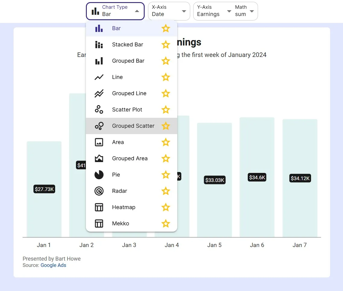 Choose between 13 chart types (all chart types are recommended for the sample data!)
The sheet opens with a chart already built from your data on the Chart tab. You can edit the following facets:
Chart Type
The chart type can be switched to bar, stacked bar, grouped bar, line, grouped line, scatter plot, grouped scatter, area, grouped area, pie, radar, heatmap or mekko.
Some chart types will be marked with a star. The stars denote recommended chart types based on the data in your spreadsheet. For example, a scatterplot will be recommended if your data contains at least 2 numerical columns.
Axis
The x and y-axis can be selected from any column in the spreadsheet. If a chart type is selected that can handle multiple series (grouped line, stacked bar, grouped area) , the y-axis dropdown will turn into a series dropdown. Using the series dropdown, you can either drill down into your data further by selecting a breakdown column, or add another series to the chart.
Some choices in the axis drop downs will be marked with a star. The star means this column is recommended for the axis based on the selected chart type. For example, date columns are recommended for the x-axis in a line chart. This will create a time series graph, and is one of the best charts to visualize changes over time. Hover over the stars to learn more reasons why a column is recommended for a particular axis.
Excel data often holds one row per transaction or record. InstaCharts aggregates the rows for you, so a sheet of individual sales can become a chart of sales by region without a pivot table. Use the Math dropdown next to the Y-axis to switch between sum, average, count, median, min and max.
Chart Text
The x-axis, y-axis, legend title and chart title auto update based on your selections. If you wish to override this text, open the Chart Text panel in the left sidebar. Subtitles, captions and source links are set there too. Axis titles, the legend and number formatting are in the Axes & Legend panel.
Chart Appearance
The chart’s width and height can be changed from the Size & Style side bar. The chart’s color scheme, fonts and theme can also be changed here.
Limit Items
Too many items appearing in the chart? New charts start with Auto Limit turned on, which keeps the 50 largest items and groups the rest into an All Others category. Turn Auto Limit off in the Data panel to choose your own number with Limit Top Items.
Filter Data
Want to restrict the data that appears in the chart? Click on the data tab and apply multiple filters per column. There is also a quick filter in the main toolbar that will filter all columns by the search term.
3. Export & Share
Use the Export dialog (located on the main toolbar) to download your chart as an image file (.png, .jpg, .svg, .webp or .pdf) or a PowerPoint slide. You can also use the Export dialog to export chart data to a csv, excel, tsv or json file.
Share charts through the Share & Templates dialog, also located on the main toolbar (sharing is an accounts only feature). You can share an interactive copy of the chart via a public link, embed it in a website, or share a static image that updates automatically when the chart changes.
Keep the chart up to date
When a newer version of the workbook arrives, right click the sheet in your workspace and choose Update Data. You can overwrite the sheet, add rows to it, or add columns to it, and your charts keep working. See Update Sheet Data for the steps.
Excel files stored in Google Drive can also stay in sync. Share the file with InstaCharts, connect it through Connect a data source in the New Sheet dialog, and upload a new version of the file in Google Drive whenever the numbers change. A paid plan can then refresh the sheet on a sync schedule.
Give it a try
InstaCharts helps you create and share professional-looking charts without writing any code. Sign up for a free account today!